A Gentle Introduction to Bayesian Statistics
The Monty Hall Problem
Introduction
Bayesian statistics has become of great interest to me and is a topic I was not really able to explore while I was in school. I think Bayesian statistics can be quite powerful with today's computing capabilities and presents a different and interesting way to tackle problems in statistics. I will attempt to present the topic in the simplest way I can. I will introduce a rather famous problem in Bayesian statistics, the Monty Hall problem. I will then first solve the problem with logic and then use Bayes' theorem to solve it. I will then solve the problem numerically with some simulations.
The Monty Hall Problem
The rules of the game are simple. There are three doors: one door has a car behind it, and the other two doors have a goat behind them. At the beggining of the game, the contestant chooses one door. Then Monty reveals what is behind one of the doors that the contestant did not choose. However, Monty knows which door has the car behind it and he will never choose that door to reveal. After Monty reveals what is behind the door, the contestant is allowed to switch his/her door with the door that Monty did not reveal. Should the contestant switch his/her door? The answer is yes, always.
Logical Explanation
At first, you might think that it makes no difference to switch doors and that there is 50⁄50 chance that the car is behind either door. But this is not true. It might seem counterintuitive that this is the case, but the key to this paradox lies in the fact that Monty will never reveal the door that has the car behind it. It turns out that after Monty reveals one of the doors that the contestant did not pick, there is a 2⁄3 chance that the car is behind the door the contestant did not choose. Let's run through all possible scenarios to demonstrate that this is the case. In addition, let's say that the contestant will always switch his/her door. Let's say the the car is behind door 1. Now let's say that the contestant chooses door 1. Monty will then randomly reveal one of the two remaining doors, since they both have goats behind them. The contestant will swtich doors and lose. Let's repeat this scenario except the contestant now chooses door 2 instead. Now Monty is forced to reveal door 3, since it is the only remaining door with a goat behind it. The contestant will switch doors and win! The same scenario as above will play out if the contestant chooses door 3. The contestant will switch doors and win as well! Thus, switching doors led the contestant to win in 2 out of 3 scenarios!
It might be useful to visualize this process as a tree diagram:
Solution using Bayes' Theorem
(This next section assumes some prerequesities - Conditional Probability, Conjoint Probability, Law of Total Probability)

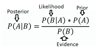
If you think way back to your college Stats 101 course, you might recognize the formula above. Yes, it is indeed the famous Bayes' theorem. What you might not recognize are the terms with arrows pointing to the different parts of the formula. This is the terminology that Bayesians used to describe the theorem.

The above image is what is known as the "diachronic" intepretation of Bayes' theorem, and also the way I like to think about Bayesian statistics. In short, in the "diachronic" intepretation of Bayesian statistics, the statistician forms hypotheses and then updates posterior probabilities based on new data/evidence. To get a better understanding, let's breakdown the above formula.
P(H) - This is simply the probability of the hypothesis before we see the data. This is often called the prior.
P(H | D) - This is what we want to calculate. Called the posterior, this is the update, the probability of the hypothesis after new data/evidence is taken into account
P(D | H) - This is called the likelihood (it is somewhat tricky to grasp at first). This is the probability of seeing the data given a
certain hypothesis. The concept of likelihood is easier to understand with some examples.ahead
P(D) - This is simply the probability of the data under any hypothesis. It is called the evidence or normalizing constant.
Now let's take one of the situations I described earlier. Let's say that the contestant chooses door 1 and that Monty subsequently reveals door 2 and there is no car there, which gives the contestant the opportunity to switch his/her door to door 3. Now let's use the "diachronic" Bayesian framework we defined earlier. Let's define all hypotheses for this scenario, that the car is behind either door 1,2, or 3. Given these hypotheses, the prior for each hypotheses is clearly 1⁄3. We made a statement about our data earlier, Monty revealed door 2 and the car was not behind it. Our statement about the data has to be clear and understood in order to define the likelihood for each hypotheses after observing the data. So if the car is truly behind door 1, then the likelihood of Monty revealing door 2 and the car not being there is 1⁄2 because the car might still be behind door 3. If the car is truly behind door 2, then the likelihood of Monty revealing door 2 and the car not being there is obviosly 0. Lastly, if the car is truly behind door 3, then the likelihood of Monty revealing door 2 and the car not being there is 1, following the logic from above.
We now have to compute the normailizing costant, P(D). Remember, this is the probability of the data under any hypothesis. In order to compute this value, we must use the law of total probability. If at most one hypothesis can be correct and there are no other possible scenarios besides the hypotheses, then we can use the law of total probability. ahead
Thus: P(D) = Σ P(Hi)P(D|Hi) = (1⁄3)(1⁄2) + (1⁄3)(0) + (1⁄3)(1) = 1⁄2
The table below summarizes our calculations:
| Prior | Likelihood | Normalizing Constant | Posterior | ||
|---|---|---|---|---|---|
| P(H) | P(D|H) | P(H)*P(D|H) | P(D) | P(H|D) | |
| 1 | 1/3 | 1/2 | 1/6 | 1/2 | 1/3 |
| 2 | 1/3 | 0 | 0 | 1/2 | 0 |
| 3 | 1/3 | 1 | 1/3 | 1/2 | 2/3 |
Thus, given our data, we have used Bayes' theorem to show that we have a 2⁄3 chance to win the car if we switch doors.
Solution using Python:
The following code represents the situation in which the contestant has chosen door 1, and Monty reveals door 2 with no prize behind it.
# defines Probability Mass Function (pmf) for the hypotheses
def Pmf(hypos):
    d = {}
    for hypo in hypos:
        d[hypo] = 1/len(hypos)
    return d

# defines Prior probabilties
def Prior(pmf,hypo):
    return pmf[hypo]

# Normalizing constant calculation
def Normalizing_Constant(pmf,data,hypos):
    total = 0
    for hypo in hypos:
        total += Prior(pmf,hypo)*Likelihood(data,hypo)
    return total

# Compute Likelihood
def Likelihood(data,hypo):
    if hypo == data:
        return 0
    elif hypo == "1":
        return 0.5
    else:
        return 1

def main():
    hypos = ["1","2","3"]
    data = "2"
    pmf = Pmf(hypos)
    print("Posterior Probabilities (P(D|H)):")
    for hypo in hypos:
        Posterior = (Prior(pmf,data)*Likelihood(data,hypo))/Normalizing_Constant(pmf,data,hypos)
        print("P({}|{}) = {}".format(data,hypo,Posterior))

if __name__ == "__main__":
    main()
Again, the logic in the code should come naturally after working through previous two sections. The likelihood function may seem a little confusing, but refer to the explanation of likelihood above to reinforce your understanding of the concept.
Results:
Posterior Probabilities (P(D|H)):
P(2|1) = 0.3333333333333333
P(2|2) = 0.0
P(2|3) = 0.6666666666666666
Conclusion:
In conclusion, the power of Bayesian statistics was used to solve a fun problem! In order to solve this paradox, we used simple logic, Bayesian statistics, and wrote a quick python script. The main takeaways from this post should be that Bayesian statistics can be a very powerful tool! Mostly that you can start with your prior beliefs and that the data can either confirm those beliefs or show you that you were wrong. While Bayesian statistics can be very powerful, one must remember that it relies heavily on assumptions. Faulty assumptions lead to inaccurate likelihood functions and will, in turn, lead to incorrect results. Nevertheless, Bayesian statistics is an exciting topic! In future posts, I plan to discuss Bayesian parameter estimation and computational methods in Bayesian statistics.